
In this post I will sketch a proof Dirichlet Theorem’s in the following form:
Theorem 1 (Dirichlet’s Theorem on Arithmetic Progression)
Let
Let 


uniformly in
Prerequisites: complex analysis, previous two posts, possibly also Dirichlet characters. It is probably also advisable to read the last chapter of Hildebrand first, since this contains a much more thorough version of an easier version in which the zeros of 
Warning: I really don’t understand what I am saying. It is at least 50% likely that this post contains a major error, and 90% likely that there will be multiple minor errors. Please kindly point out any screw-ups of mine; thanks!
Throughout this post: 


1. Outline
Here are the main steps:
- We introduce Dirichlet character
which will serves as a roots of unity filter, extracting terms
. We will see that this reduces the problem to estimating the function
.
- Introduce the
, the generalization of
for arithmetic progressions. Establish a functional equation in terms of
, much like with
to a meromorphic function in the entire complex plane.
- We will use a variation on the Perron transformation in order to transform this sum into an integral involving an
. We truncate this integral to
; this introduces an error
that can be computed immediately, though in this presentation we delay its computation until later.
- We do a contour as in the proof of the Prime Number Theorem in order to estimate the above integral in terms of the zeros of
. The main term emerges as a residue, so we want to show that the integral
along this integral goes to zero. Moreover, we get some residues
related to the zeros of the
- By using Hadamard’s Theorem on
in terms of its zeros. This has three consequences:
- We can use the previous to get bounds on
.
- Using a 3-4-1 trick, this gives us information on the horizontal distribution of
; the dreaded Siegel zeros appear here.
- We can get an expression which lets us estimate the vertical distribution of the zeros in the critical strip (specifically the number of zeros with
).
The first and third points let us compute
- We can use the previous to get bounds on
- The horizontal zero-free region gives us an estimate of
.
- We use Siegel’s Theorem to handle the potential Siegel zero that might arise.
Possibly helpful diagram:

The pink dots denote zeros; we think the nontrivial ones all lie on the half-line by the Generalized Riemann Hypothesis but they could actually be anywhere in the green strip.
2. Dirichlet Characters
2.1. Definitions
Recall that a Dirichlet character 


In particular, 


If 


2.2. Orthogonality
The key fact about Dirichlet characters which will enable us to prove the theorem is the following trick:
Theorem 2 (Orthogonality of Dirichlet Characters)
We have
(Here 
This is in some senses a slightly fancier form of the old roots of unity filter. Specifically, it is not too hard to show that 


2.3. Dirichlet -Functions
Now we can define the associated

The properties of these
Theorem 3
Let
- If
,
.
- If
,
of residue
.
The proof is pretty much the same as for zeta.
Observe that if 

2.4. The Functional Equation for Dirichlet -Functions
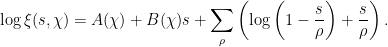
While I won’t prove it here, one can show the following analog of the functional equation for Dirichlet
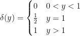
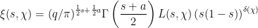
Theorem 4 (The Functional Equation of Dirichlet
Assume that 

![\displaystyle \xi(s,\chi) = q^{\frac{1}{2}(s+a)} \gamma(s,\chi) L(s,\chi) \left[ s(1-s) \right]^{\delta(x)}](https://s0.wp.com/latex.php?latex=%5Cdisplaystyle+%5Cxi%28s%2C%5Cchi%29+%3D+q%5E%7B%5Cfrac%7B1%7D%7B2%7D%28s%2Ba%29%7D+%5Cgamma%28s%2C%5Cchi%29+L%28s%2C%5Cchi%29+%5Cleft%5B+s%281-s%29+%5Cright%5D%5E%7B%5Cdelta%28x%29%7D+&bg=ffffff&fg=000000&s=0&c=20201002)
where
and 
is entire.
- If
for some complex number
.
Unlike the 
- For
,
,
and so on.
- For
even, we get zeros at
,
at
is no longer canceled).
- For
,
,
and so on.
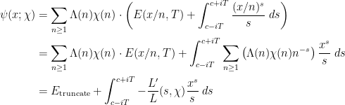
3. Obtaining the Contour Integral
3.1. Orthogonality
Using the trick of orthogonality, we may write
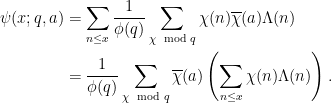
To do this we have to estimate the sum 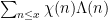
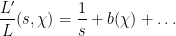
3.2. Introducing the Logarithmic Derivative of the -Function
First, we realize 


Taking the derivative, we obtain
Theorem 5
For any

Proof:
as desired.

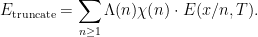
3.3. The Truncation Trick
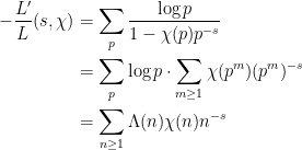
Now, we unveil the trick at the heart of the proof of Perron’s Formula in the last post. I will give a more precise statement this time, by stating where this integral comes from:
Lemma 6 (Truncated Version of Perron Lemma)
For any 
Then 

and the error term 
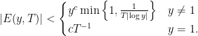
In particular, 
In effect, the integral from 


3.4. Applying the Truncation
Let’s do so: define

which is almost the same as 


where
Estimating this is quite ugly, so we defer it to later.
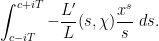
4. Applying the Residue Theorem
4.1. Primitive Characters
Exactly like before, we are going to use a contour to estimate the value of
Let 


During this process we pick up residues, which are the interesting terms.
First, assume that
- If
corresponding to
This is the “main term”. Per laziness,
it is.
- Depending on whether
Actually, I really ought to truncate this at
in a moment I really don’t want to take the time to do so; the difference is negligible.
- We obtain a residue of
, which we denote
, for
straight-out.
- If
and notice that
so we pick up an extra residue of
. So, call this a bonus of
- Finally, the hard-to-understand zeros in the strip
. If
is a zero, then it contributes a residue of
. We only pick up the zeros with
in our rectangle, so we get a term


Letting

at least for primitive characters. Note that the sum over the zeros is not absolutely convergent without the restriction to
4.2. Transition to nonprimitive characters
The next step is to notice that if 

and so our above formula in fact holds for any character 

Anyways

Thus we have
Unfortunately, the constant
5. Distribution of Zeros
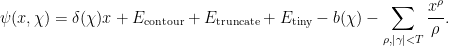
In order to estimate

we will need information on both the vertical and horizontal distribution of the zeros. Also, it turns out this will help us compute
5.1. Applying Hadamard’s Theorem
Let
is entire. It also is easily seen to have order 


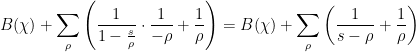
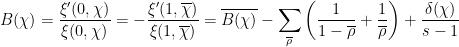
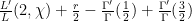
Taking a logarithmic derivative and cleaning up, we derive the following lemma.
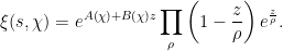
Lemma 7 (Hadamard Expansion of Logarithmic Derivative)
For any primitive character
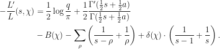
Proof: One one hand, we have
On the other hand

Taking the derivative of both sides and setting them equal: we have on the left side
and on the right-hand side

Equating these gives the desired result.
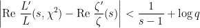
This will be useful in controlling things later. The 
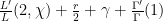
5.2. A Bound on the Logarithmic Derivative
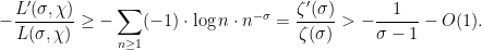
Frequently we will take the real part of this. Using Stirling, the short version of this is:
Lemma 8 (Logarithmic Derivative Bound)
Let 
![\displaystyle \text{Re } \left[ -\frac{L'(\sigma+it, \chi)}{L(\sigma+it, \chi)} \right] = \begin{cases} O(\mathcal L) - \text{Re } \sum_\rho \frac{1}{s-\rho} + \text{Re } \frac{\delta(\chi)}{s-1} & 1 \le \sigma \le 2 \\ O(\mathcal L) - \text{Re } \sum_\rho \frac{1}{s-\rho} & 1 \le \sigma \le 2, \left\lvert t \right\rvert \ge 2 \\ O(1) & \sigma \ge 2. \end{cases}](https://s0.wp.com/latex.php?latex=%5Cdisplaystyle+%5Ctext%7BRe+%7D+%5Cleft%5B+-%5Cfrac%7BL%27%28%5Csigma%2Bit%2C+%5Cchi%29%7D%7BL%28%5Csigma%2Bit%2C+%5Cchi%29%7D+%5Cright%5D+%3D+%5Cbegin%7Bcases%7D+O%28%5Cmathcal+L%29+-+%5Ctext%7BRe+%7D+%5Csum_%5Crho+%5Cfrac%7B1%7D%7Bs-%5Crho%7D+%2B+%5Ctext%7BRe+%7D+%5Cfrac%7B%5Cdelta%28%5Cchi%29%7D%7Bs-1%7D+%26+1+%5Cle+%5Csigma+%5Cle+2+%5C%5C+O%28%5Cmathcal+L%29+-+%5Ctext%7BRe+%7D+%5Csum_%5Crho+%5Cfrac%7B1%7D%7Bs-%5Crho%7D+%26+1+%5Cle+%5Csigma+%5Cle+2%2C+%5Cleft%5Clvert+t+%5Cright%5Crvert+%5Cge+2+%5C%5C+O%281%29+%26+%5Csigma+%5Cge+2.+%5Cend%7Bcases%7D+&bg=ffffff&fg=000000&s=0&c=20201002)
Proof: The claim is obvious for 


where 
First, we claim that 
where the ends come from taking the logarithmic derivative directly. By switching 
Then, the lemma follows rather directly; the 


and the first two terms contribute 


Short version: our functional equation lets us relate 

Lemma 9 (Far-Left Estimate of Log Derivative)
If 

![\displaystyle \frac{L'(s, \chi)}{L(s, \chi)} = O\left[ \log q\left\lvert s \right\rvert \right].](https://s0.wp.com/latex.php?latex=%5Cdisplaystyle+%5Cfrac%7BL%27%28s%2C+%5Cchi%29%7D%7BL%28s%2C+%5Cchi%29%7D+%3D+O%5Cleft%5B+%5Clog+q%5Cleft%5Clvert+s+%5Cright%5Crvert+%5Cright%5D.+&bg=ffffff&fg=000000&s=0&c=20201002)
Proof:
We have

(the unsymmetric functional equation, which can be obtained from Legendre’s duplication formula). Taking a logarithmic derivative yields

Because we assumed 


5.3. Horizontal Distribution
I claim that:
Theorem 10 (Horizontal Distribution Bound)
Let 
- If
.
- If
Such bad zeros are called Siegel zeros, and I will denote them 
Proof: First, assume
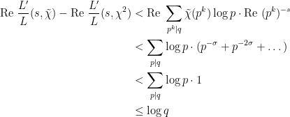
By the 3-4-1 lemma on 
![\displaystyle 3 \text{Re } \left[ -\frac{L'(\sigma, \chi_0)}{L(\sigma, \chi_0)} \right] + 4 \text{Re } \left[ -\frac{L'(\sigma+it, \chi)}{L(\sigma+it, \chi)} \right] + \text{Re } \left[ -\frac{L'(\sigma+2it, \chi^2)}{L(\sigma+2it, \chi^2)} \right] \ge 0.](https://s0.wp.com/latex.php?latex=%5Cdisplaystyle+3+%5Ctext%7BRe+%7D+%5Cleft%5B+-%5Cfrac%7BL%27%28%5Csigma%2C+%5Cchi_0%29%7D%7BL%28%5Csigma%2C+%5Cchi_0%29%7D+%5Cright%5D+%2B+4+%5Ctext%7BRe+%7D+%5Cleft%5B+-%5Cfrac%7BL%27%28%5Csigma%2Bit%2C+%5Cchi%29%7D%7BL%28%5Csigma%2Bit%2C+%5Cchi%29%7D+%5Cright%5D+%2B+%5Ctext%7BRe+%7D+%5Cleft%5B+-%5Cfrac%7BL%27%28%5Csigma%2B2it%2C+%5Cchi%5E2%29%7D%7BL%28%5Csigma%2B2it%2C+%5Cchi%5E2%29%7D+%5Cright%5D+%5Cge+0.+&bg=ffffff&fg=000000&s=0&c=20201002)
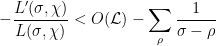
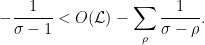
This is cool because we already know that
![\displaystyle \text{Re } \left[ -\frac{L'(\sigma+it, \chi)}{L(\sigma+it, \chi)} \right] < O(\mathcal L) - \text{Re } \sum_\rho \frac{1}{s-\rho}](https://s0.wp.com/latex.php?latex=%5Cdisplaystyle+%5Ctext%7BRe+%7D+%5Cleft%5B+-%5Cfrac%7BL%27%28%5Csigma%2Bit%2C+%5Cchi%29%7D%7BL%28%5Csigma%2Bit%2C+%5Cchi%29%7D+%5Cright%5D+%3C+O%28%5Cmathcal+L%29+-+%5Ctext%7BRe+%7D+%5Csum_%5Crho+%5Cfrac%7B1%7D%7Bs-%5Crho%7D+&bg=ffffff&fg=000000&s=0&c=20201002)
We now assume 
In particular, we now have (since 

So we are free to throw out as many terms as we want.
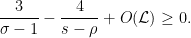
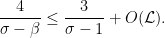
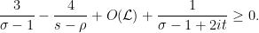
If 
![\displaystyle \begin{aligned} \text{Re } \left[ -\frac{L'(\sigma, \chi_0)}{L(\sigma, \chi_0)} \right] &\le \frac{1}{\sigma-1} + O(1) \\ \text{Re } \left[ -\frac{L'(\sigma+it, \chi)}{L(\sigma+it, \chi)} \right] &\le O(\mathcal L) - \frac{1}{s-\rho} \\ \text{Re } \left[ -\frac{L'(\sigma+2it, \chi^2)}{L(\sigma+2it, \chi^2)} \right] &\le O(\mathcal L) \end{aligned}](https://s0.wp.com/latex.php?latex=%5Cdisplaystyle+%5Cbegin%7Baligned%7D+%5Ctext%7BRe+%7D+%5Cleft%5B+-%5Cfrac%7BL%27%28%5Csigma%2C+%5Cchi_0%29%7D%7BL%28%5Csigma%2C+%5Cchi_0%29%7D+%5Cright%5D+%26%5Cle+%5Cfrac%7B1%7D%7B%5Csigma-1%7D+%2B+O%281%29+%5C%5C+%5Ctext%7BRe+%7D+%5Cleft%5B+-%5Cfrac%7BL%27%28%5Csigma%2Bit%2C+%5Cchi%29%7D%7BL%28%5Csigma%2Bit%2C+%5Cchi%29%7D+%5Cright%5D+%26%5Cle+O%28%5Cmathcal+L%29+-+%5Cfrac%7B1%7D%7Bs-%5Crho%7D+%5C%5C+%5Ctext%7BRe+%7D+%5Cleft%5B+-%5Cfrac%7BL%27%28%5Csigma%2B2it%2C+%5Cchi%5E2%29%7D%7BL%28%5Csigma%2B2it%2C+%5Cchi%5E2%29%7D+%5Cright%5D+%26%5Cle+O%28%5Cmathcal+L%29+%5Cend%7Baligned%7D+&bg=ffffff&fg=000000&s=0&c=20201002)
where we have dropped all but one term for the second line, and all terms for the third line. If 
just like earlier: 
Consequently, we derive using 
Selecting 

If we select 
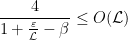
so

for some constant 
But because the Euler product of the 
Unfortunately, if we are unlucky enough that 
Applied with 
If 


for any 
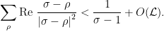
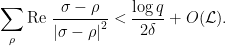
Now let’s examine 

where we no longer need the real parts since
So
In other words,
Then, let 
The rest is arithmetic; basically one finds that there can be at most one Siegel zero. In particular, since complex zeros come in conjugate pairs, that zero must be real.
It remains to handle the case that
5.4. Vertical Distribution
We have the following lemma:
Lemma 11 (Sum of Zeros Lemma)
For all real 
Proof: We already have that

and we take 

as needed.
From this we may deduce that
Lemma 12 (Number of Zeros Nearby
For all real ![{\gamma \in [t-1, t+1]}](https://s0.wp.com/latex.php?latex=%7B%5Cgamma+%5Cin+%5Bt-1%2C+t%2B1%5D%7D&bg=ffffff&fg=000000&s=0&c=20201002)

In particular, we may perturb any given 


From this, using an argument principle we can actually also obtain the following: For a real number 

![{\gamma \in [-T, T]}](https://s0.wp.com/latex.php?latex=%7B%5Cgamma+%5Cin+%5B-T%2C+T%5D%7D&bg=ffffff&fg=000000&s=0&c=20201002)
6. Error Term Party
Up to now, 


so 

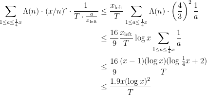
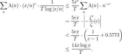
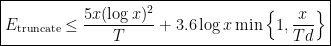
6.1. Estimating the Truncation Error
Recall that
We need to bound the right-hand side of

If 


We let 


So we have possibly a center term (if 

- In the easy case, if
, which is piddling (less than
).
- Suppose
. If
for some integer
, then
by using the silly inequality
for
. So the contribution in total is at most
provided
.
- If
, we have
Hence in this case, we get an error at most
- The cases
and
give the same bounds as above, in the same way.


Finally, if for 
(Recall 
The sum of everything is 
provided 
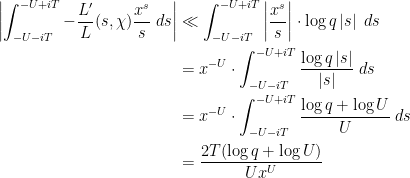
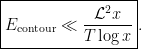
6.2. Estimating the Contour Error
We now need to measure the error along the contour, taken from 

For this we appeal to the Hadamard expansion. We break into a couple cases.
- First, let’s look at the integral when
, so
with
Thus we want an estimate of
.
Lemma 13
Let
of any zeros of
Proof: Since we assumed that
and so we obtain
and we eliminate
where
by Stirling (here we use the fact that
we see that
So the contribution of the sum for
can be bounded by
As for the zeros with smaller imaginary part, we at least have
and thus we can reduce the sum to just
Now by the assumption that
; so the terms of the sum are all at most
is bounded; we can write it using its (convergent) Dirichlet series and then note it is at most
.
At this point, we perturb - Next, for the integral
, we use the “far-left” estimate to obtain
So the contribution in this case is
.
- Along the horizontal integral, we can use the same bound
which vanishes as


![\displaystyle \frac{L'(\sigma+it, \chi)}{L(\sigma+it, \chi)} - \frac{L'(2+it, \chi)}{L(2+it, \chi)} = \sum_{\gamma\in[t-1,t+1]} \frac{1}{\sigma+it-\rho} + O(\mathcal L).](https://s0.wp.com/latex.php?latex=%5Cdisplaystyle+%5Cfrac%7BL%27%28%5Csigma%2Bit%2C+%5Cchi%29%7D%7BL%28%5Csigma%2Bit%2C+%5Cchi%29%7D+-+%5Cfrac%7BL%27%282%2Bit%2C+%5Cchi%29%7D%7BL%282%2Bit%2C+%5Cchi%29%7D+%3D+%5Csum_%7B%5Cgamma%5Cin%5Bt-1%2Ct%2B1%5D%7D+%5Cfrac%7B1%7D%7B%5Csigma%2Bit-%5Crho%7D+%2B+O%28%5Cmathcal+L%29.+&bg=ffffff&fg=000000&s=0&c=20201002)


So we only have two error terms, 

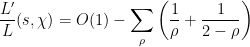
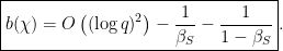
6.3. The term
We can estimate
Lemma 14
For primitive
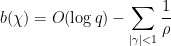
Proof: The idea is to look at 

Then at
where the 

which is 

This completes the proof.
Let 

. Then
; since
is a zero of
is a zero of
. Moreover, in the range
there are
in our earlier lemma on vertical distribution).
Thus, total contribution of the sum is 
- If
, then
. We pull these terms out separately.Consequently,
By adjusting the constant, we may assume
if it exists.
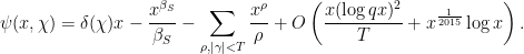
7. Computing
7.1. Summing the Error Terms
We now have, for any
where
Assume now that
, and
). Then aggregating all the errors gives
where the sum over
, and also
Absorbing things into the error term,
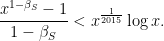
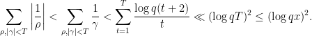
7.2. Estimating the Sum Over Zeros
Now we want to estimate
We do this is the dumbest way possible: putting a bound on
and pulling it out.
For any non-Siegel zero, we have a zero-free region
, whence
Pulling this out, we can then estimate the reciprocals by using our differential:
Hence,
We select
for some constant
, and moreover assume
, then we obtain
7.3. Summing Up
We would like to sum over all characters
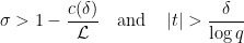
Theorem 15 (Landau)
If
and
are real nontrivial primitive characters modulo
and
, then for any zeros
we have
for some fixed absolute
. In particular, for any fixed
with a Siegel zero.
Proof: The character
is not trivial, so we can put
Now we use a silly trick:
by “Simon’s Favorite Factoring Trick” (we use the deep fact that
, the analog of
and one may deduce the conclusion from here.
We now sum over all characters
where
is the character with a Siegel zero, if it exists.
8. Siegel’s Theorem, and Finishing Off
The term with
is bad, and we need some way to get rid of it. We now appeal to Siegel’s Theorem:
Theorem 16 (Siegel’s Theorem)
For any
there is a
such that any Siegel zero
Thus for a positive constant
means
, so we obtain
Then
where
. This completes the proof of Dirichlet’s Theorem.


Slight typo: the entry title says “Dircihlet” instead of “Dirichlet”.
Also, the first sentence “In this post I will sketch a proof Dirichlet Theorem’s in the following form:” doesn’t make sense lol.
LikeLike
Thanks, I’ve fixed that. And yes, it was originally supposed to be a sketch but got longer than that…
LikeLike
No, what I meant was there was a missing “of” or something to that effect.
In any case, do you happen to know the “strongest” form of Dirichlet’s theorem that can be proven using elementary methods?
LikeLike
I don’t know of any elementary (non-analytic) methods that get useful forms of Dirichlet’s Theorem. The closest I know of is showing that there are infinitely many primes , by plugging things in to the
  th cyclotomic polynomial.
LikeLike
Isn’t this the Siegel-Walfisz Theorem? I thought Dirichlet’s Theorem was the one that stated that there are infinitely many primes in arithmetic progressions (excluding the trivial cases).
LikeLike
Fair point, you’re right of course. :) I usually just call it Dirichlet just because everyone knows immediately what it means, whereas I’m never heard of the name “Siegel-Walfisz” until now. (I hear it called PNT for Arithmetic Progressions, though.)
LikeLike
[…] I talked about last time on my blog, the key ingredients […]
LikeLike