A trailer for p-adic analysis, first half: USA TST 2003

I think this post is more than two years late in coming, but anywhow…

This post introduces the ${p}$ -adic integers ${\mathbb Z_p}$ , and the ${p}$ -adic numbers ${\mathbb Q_p}$ . The one-sentence description is that these are “integers/rationals carrying full mod ${p^e}$ information” (and only that information).

The first four sections will cover the founding definitions culminating in a short solution to a USA TST problem.

In this whole post, ${p}$ is always a prime. Much of this is based off of Chapter 3A from Straight from the Book.

1. Motivation

Before really telling you what ${\mathbb Z_p}$ and ${\mathbb Q_p}$ are, let me tell you what you might expect them to do.

In elementary/olympiad number theory, we’re already well-familiar with the following two ideas:

Taking modulo a prime ${p}$ or prime ${p^e}$ , and
Looking at the exponent ${\nu_p}$ .

Let me expand on the first point. Suppose we have some Diophantine equation. In olympiad contexts, one can take an equation modulo ${p}$ to gain something else to work with. Unfortunately, taking modulo ${p}$ loses some information: (the reduction ${\mathbb Z \twoheadrightarrow \mathbb Z/p}$ is far from injective).

If we want finer control, we could consider instead taking modulo ${p^2}$ , rather than taking modulo ${p}$ . This can also give some new information (cubes modulo ${9}$ , anyone?), but it has the disadvantage that ${\mathbb Z/p^2}$ isn’t a field, so we lose a lot of the nice algebraic properties that we got if we take modulo ${p}$ .

One of the goals of ${p}$ -adic numbers is that we can get around these two issues I described. The ${p}$ -adic numbers we introduce is going to have the following properties:

You can “take modulo ${p^e}$ for all ${e}$ at once”. In olympiad contexts, we are used to picking a particular modulus and then seeing what happens if we take that modulus. But with ${p}$ -adic numbers, we won’t have to make that choice. An equation of ${p}$ -adic numbers carries enough information to take modulo ${p^e}$ .
The numbers ${\mathbb Q_p}$ form a field, the nicest possible algebraic structure: ${1/p}$ makes sense. Contrast this with ${\mathbb Z/p^2}$ , which is not even an integral domain.
It doesn’t lose as much information as taking modulo ${p}$ does: rather than the surjective ${\mathbb Z \twoheadrightarrow \mathbb Z/p}$ we have an injective map ${\mathbb Z \hookrightarrow \mathbb Z_p}$ .
Despite this, you “ignore” some “irrelevant” data. Just like taking modulo ${p}$ , you want to zoom-in on a particular type of algebraic information, and this means necessarily losing sight of other things. (To draw an analogy: the equation ${ a^2 + b^2 + c^2 + d^2 = -1}$ has no integer solutions, because, well, squares are nonnegative. But you will find that this equation has solutions modulo any prime ${p}$ , because once you take modulo ${p}$ you stop being able to talk about numbers being nonnegative. The same thing will happen if we work in ${p}$ -adics: the above equation has a solution in ${\mathbb Z_p}$ for every prime ${p}$ .)

So, you can think of ${p}$ -adic numbers as the right tool to use if you only really care about modulo ${p^e}$ information, but normal ${\mathbb Z/p^e}$ isn’t quite powerful enough.

To be more concrete, I’ll give a poster example now:

Example 1 (USA TST 2002/2)

For a prime ${p}$ , show the value of

$\displaystyle f_p(x) = \sum_{k=1}^{p-1} \frac{1}{(px+k)^2} \pmod{p^3}$

does not depend on ${x}$ .

Here is a problem where we clearly only care about ${p^e}$ -type information. Yet it’s a nontrivial challenge to do the necessary manipulations mod ${p^3}$ (try it!). The basic issue is that there is no good way to deal with the denominators modulo ${p^3}$ (in part ${\mathbb Z/p^3}$ is not even an integral domain).

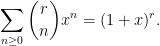
However, with ${p}$ -adic analysis we’re going to be able to overcome these limitations and give a “straightforward” proof by using the identity

$\displaystyle \left( 1 + \frac{px}{k} \right)^{-2} = \sum_{n \ge 0} \binom{-2}{n} \left( \frac{px}{k} \right)^n.$

Such an identity makes no sense over ${\mathbb Q}$ or ${\mathbb R}$ for converge reasons, but it will work fine over the ${\mathbb Q_p}$ , which is all we need.

2. Algebraic perspective

We now construct ${\mathbb Z_p}$ and ${\mathbb Q_p}$ . I promised earlier that a ${p}$ -adic integer will let you look at “all residues modulo ${p^e}$ ” at once. This definition will formalize this.

2.1. Definition of ${\mathbb Z_p}$

Definition 2 (Introducing ${\mathbb Z_p}$ )

A ${p}$ -adic integer is a sequence

$\displaystyle x = (x_1 \bmod p, \; x_2 \bmod{p^2}, \; x_3 \bmod{p^3}, \; \dots)$

of residues ${x_e}$ modulo ${p^e}$ for each integer ${e}$ , satisfying the compatibility relations ${x_i \equiv x_j \pmod{p^i}}$ for ${i < j}$ .

The set ${\mathbb Z_p}$ of ${p}$ -adic integers forms a ring under component-wise addition and multiplication.

Example 3 (Some ${3}$ -adic integers)

Let ${p=3}$ . Every usual integer ${n}$ generates a (compatible) sequence of residues modulo ${p^e}$ for each ${e}$ , so we can view each ordinary integer as ${p}$ -adic one:

$\displaystyle 50 = \left( 2 \bmod 3, \; 5 \bmod 9, \; 23 \bmod{27}, \; 50 \bmod{81}, \; 50 \bmod{243}, \; \dots \right).$

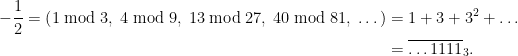
On the other hand, there are sequences of residues which do not correspond to any usual integer despite satisfying compatibility relations, such as

$\displaystyle \left( 1 \bmod 3, \; 4 \bmod 9, \; 13 \bmod{27}, \; 40 \bmod{81}, \; \dots \right)$

which can be thought of as ${x = 1 + p + p^2 + \dots}$ .

In this way we get an injective map

$\displaystyle \mathbb Z \hookrightarrow \mathbb Z_p \qquad n \mapsto \left( n \bmod p, n \bmod{p^2}, n \bmod{p^3}, \dots \right)$

which is not surjective. So there are more ${p}$ -adic integers than usual integers.

(Remark for experts: those of you familiar with category theory might recognize that this definition can be written concisely as

$\displaystyle \mathbb Z_p \overset{\mathrm{def}}{=} \varprojlim \mathbb Z/p^e \mathbb Z$

where the inverse limit is taken across ${e \ge 1}$ .)

Exercise 4

Check that ${\mathbb Z_p}$ is an integral domain.

2.2. Base ${p}$ expansion

Here is another way to think about ${p}$ -adic integers using “base ${p}$ ”. As in the example earlier, every usual integer can be written in base ${p}$ , for example

$\displaystyle 50 = \overline{1212}_3 = 2 \cdot 3^0 + 1 \cdot 3^1 + 2 \cdot 3^2 + 1 \cdot 3^3.$

More generally, given any ${x = (x_1, \dots) \in \mathbb Z_p}$ , we can write down a “base ${p}$ ” expansion in the sense that there are exactly ${p}$ choices of ${x_k}$ given ${x_{k-1}}$ . Continuing the example earlier, we would write

$\displaystyle \begin{aligned} \left( 1 \bmod 3, \; 4 \bmod 9, \; 13 \bmod{27}, \; 40 \bmod{81}, \; \dots \right) &= 1 + 3 + 3^2 + \dots \\ &= \overline{\dots1111}_3 \end{aligned}$

and in general we can write

$\displaystyle x = \sum_{k \ge 0} a_k p^k = \overline{\dots a_2 a_1 a_0}_p$

where ${a_k \in \{0, \dots, p-1\}}$ , such that the equation holds modulo ${p^e}$ for each ${e}$ . Note the expansion is infinite to the left, which is different from what you’re used to.

(Amusingly, negative integers also have infinite base ${p}$ expansions: ${-4 = \overline{\dots222212}_3}$ , corresponding to ${(2 \bmod 3, \; 5 \bmod 9, \; 23 \bmod{27}, \; 77 \bmod{81} \dots)}$ .)

Thus you may often hear the advertisement that a ${p}$ -adic integer is an “possibly infinite base ${p}$ expansion”. This is correct, but later on we’ll be thinking of ${\mathbb Z_p}$ in a more and more “analytic” way, and so I prefer to think of this as a “Taylor series with base ${p}$ ”. Indeed, much of your intuition from generating functions ${K[[X]]}$ (where ${K}$ is a field) will carry over to ${\mathbb Z_p}$ .

2.3. Constructing ${\mathbb Q_p}$

Here is one way in which your intuition from generating functions carries over:

Proposition 5 (Non-multiples of ${p}$ are all invertible)

The number ${x \in \mathbb Z_p}$ is invertible if and only if ${x_1 \ne 0}$ . In symbols,

$\displaystyle x \in \mathbb Z_p^\times \iff x \not\equiv 0 \pmod p.$

Contrast this with the corresponding statement for ${K[ [ X ] ]}$ : a generating function ${F \in K[ [ X ] ]}$ is invertible iff ${F(0) \neq 0}$ .

Proof: If ${x \equiv 0 \pmod p}$ then ${x_1 = 0}$ , so clearly not invertible. Otherwise, ${x_e \not\equiv 0 \pmod p}$ for all ${e}$ , so we can take an inverse ${y_e}$ modulo ${p^e}$ , with ${x_e y_e \equiv 1 \pmod{p^e}}$ . As the ${y_e}$ are themselves compatible, the element ${(y_1, y_2, \dots)}$ is an inverse. $\Box$

Example 6 (We have ${-\frac{1}{2} = \overline{\dots1111}_3 \in \mathbb Z_3}$ )

We claim the earlier example is actually

$\displaystyle \begin{aligned} -\frac{1}{2} = \left( 1 \bmod 3, \; 4 \bmod 9, \; 13 \bmod{27}, \; 40 \bmod{81}, \; \dots \right) &= 1 + 3 + 3^2 + \dots \\ &= \overline{\dots1111}_3. \end{aligned}$

Indeed, multiplying it by ${-2}$ gives

$\displaystyle \left( -2 \bmod 3, \; -8 \bmod 9, \; -26 \bmod{27}, \; -80 \bmod{81}, \; \dots \right) = 1.$

(Compare this with the “geometric series” ${1 + 3 + 3^2 + \dots = \frac{1}{1-3}}$ . We’ll actually be able to formalize this later, but not yet.)

Remark 7 ( ${\frac{1}{2}}$ is an integer for ${p > 2}$ )

The earlier proposition implies that ${\frac{1}{2} \in \mathbb Z_3}$ (among other things); your intuition about what is an “integer” is different here! In olympiad terms, we already knew ${\frac{1}{2} \pmod 3}$ made sense, which is why calling ${\frac{1}{2}}$ an “integer” in the ${3}$ -adics is correct, even though it doesn’t correspond to any element of ${\mathbb Z}$ .

Fun (but trickier) exercise: rational numbers correspond exactly to eventually periodic base ${p}$ expansions.

With this observation, here is now the definition of ${\mathbb Q_p}$ .

Definition 8 (Introducing ${\mathbb Q_p}$ )

Since ${\mathbb Z_p}$ is an integral domain, we let ${\mathbb Q_p}$ denote its field of fractions. These are the ${p}$ -adic numbers.

Continuing our generating functions analogy:

$\displaystyle \mathbb Z_p \text{ is to } \mathbb Q_p \quad\text{as}\quad K[[X]] \text{ is to } K((X)).$

This means ${\mathbb Q_p}$ is “Laurent series with base ${p}$ ”, and in particular according to the earlier proposition we deduce:

Proposition 9 ( ${\mathbb Q_p}$ looks like formal Laurent series)

Every nonzero element of ${\mathbb Q_p}$ is uniquely of the form

$\displaystyle p^k u \qquad \text{ where } k \in \mathbb Z, \; u \in \mathbb Z_p^\times.$

Thus, continuing our base ${p}$ analogy, elements of ${\mathbb Q_p}$ are in bijection with “Laurent series”

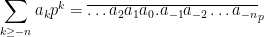
$\displaystyle \sum_{k \ge -n} a_k p^k = \overline{\dots a_2 a_1 a_0 . a_{-1} a_{-2} \dots a_{-n}}_p$

for ${a_k \in \left\{ 0, \dots, p-1 \right\}}$ . So the base ${p}$ representations of elements of ${\mathbb Q_p}$ can be thought of as the same as usual, but extending infinitely far to the left (rather than to the right).

(Fair warning: the field ${\mathbb Q_p}$ has characteristic zero, not ${p}$ .)

Remark 10 (Warning on fraction field)

This result implies that you shouldn’t think about elements of ${\mathbb Q_p}$ as ${x/y}$ (for ${x,y \in \mathbb Z_p}$ ) in practice, even though this is the official definition (and what you’d expect from the name ${\mathbb Q_p}$ ). The only denominators you need are powers of ${p}$ .

To keep pushing the formal Laurent series analogy, ${K((X))}$ is usually not thought of as quotient of generating functions but rather as “formal series with some negative exponents”. You should apply the same intuition on ${\mathbb Q_p}$ .

(At this point I want to make a remark about the fact ${1/p \in \mathbb Q_p}$ , connecting it to the wish-list of properties I had before. In elementary number theory you can take equations modulo ${p}$ , but if you do the quantity ${n/p \bmod{p}}$ doesn’t make sense unless you know ${n \bmod{p^2}}$ . You can’t fix this by just taking modulo ${p^2}$ since then you need ${n \bmod{p^3}}$ to get ${n/p \bmod{p^2}}$ , ad infinitum. You can work around issues like this, but the nice feature of ${\mathbb Z_p}$ and ${\mathbb Q_p}$ is that you have modulo ${p^e}$ information for “all ${e}$ at once”: the information of ${x \in \mathbb Q_p}$ packages all the modulo ${p^e}$ information simultaneously. So you can divide by ${p}$ with no repercussions.)

3. Analytic perspective

3.1. Definition

Up until now we’ve been thinking about things mostly algebraically, but moving forward it will be helpful to start using the language of analysis. Usually, two real numbers are considered “close” if they are close on the number of line, but for ${p}$ -adic purposes we only care about modulo ${p^e}$ information. So, we’ll instead think of two elements of ${\mathbb Z_p}$ or ${\mathbb Q_p}$ as “close” if they differ by a large multiple of ${p^e}$ .

For this we’ll borrow the familiar ${\nu_p}$ from elementary number theory.

Definition 11 ( ${p}$ -adic valuation and absolute value)

We define the ${p}$ -adic valuation ${\nu_p : \mathbb Q_p^\times \rightarrow \mathbb Z}$ in the following two equivalent ways:

For ${x = (x_1, x_2, \dots) \in \mathbb Z_p}$ we let ${\nu_p(x)}$ be the largest ${e}$ such that ${x_e \equiv 0 \pmod{p^e}}$ (or ${e=0}$ if ${x \in \mathbb Z_p^\times}$ ). Then extend to all of ${\mathbb Q_p^\times}$ by ${\nu_p(xy) = \nu_p(x) + \nu_p(y)}$ .
Each ${x \in \mathbb Q_p^\times}$ can be written uniquely as ${p^k u}$ for ${u \in \mathbb Z_p^\times}$ , ${k \in \mathbb Z}$ . We let ${\nu_p(x) = k}$ .

By convention we set ${\nu_p(0) = +\infty}$ . Finally, define the ${p}$ -adic absolute value ${\left\lvert \bullet \right\rvert_p}$ by

$\displaystyle \left\lvert x \right\rvert_p = p^{-\nu_p(x)}.$

In particular ${\left\lvert 0 \right\rvert_p = 0}$ .

This fulfills the promise that ${x}$ and ${y}$ are close if they look the same modulo ${p^e}$ for large ${e}$ ; in that case ${\nu_p(x-y)}$ is large and accordingly ${\left\lvert x-y \right\rvert_p}$ is small.

3.2. Ultrametric space

In this way, ${\mathbb Q_p}$ and ${\mathbb Z_p}$ becomes a metric space with metric given by ${\left\lvert x-y \right\rvert_p}$ .

Exercise 12

Suppose ${f \colon \mathbb Z_p \rightarrow \mathbb Q_p}$ is continuous and ${f(n) = (-1)^n}$ for every ${n \in \mathbb Z_{\ge 0}}$ . Prove that ${p = 2}$ .

In fact, these spaces satisfy a stronger form of the triangle inequality than you are used to from ${\mathbb R}$ .

Proposition 13 ( ${\left\lvert \bullet \right\rvert_p}$ is an ultrametric)

For any ${x,y \in \mathbb Z_p}$ , we have the strong triangle inequality

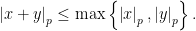
$\displaystyle \left\lvert x+y \right\rvert_p \le \max \left\{ \left\lvert x \right\rvert_p, \left\lvert y \right\rvert_p \right\}.$

Equality holds if (but not only if) ${\left\lvert x \right\rvert_p \neq \left\lvert y \right\rvert_p}$ .

However, ${\mathbb Q_p}$ is more than just a metric space: it is a field, with its own addition and multiplication. This means we can do analysis just like in ${\mathbb R}$ or ${\mathbb C}$ : basically, any notion such as “continuous function”, “convergent series”, et cetera has a ${p}$ -adic analog. In particular, we can define what it means for an infinite sum to converge:

Definition 14 (Convergence notions)

Here are some examples of ${p}$ -adic analogs of “real-world” notions.

A sequence ${s_1}$ , \dots converges to a limit ${L}$ if ${\lim_{n \rightarrow \infty} \left\lvert s_n - L \right\rvert_p = 0}$ .
The infinite series ${\sum_k x_k}$ converges if the sequence of partial sums ${s_1 = x_1}$ , ${s_2 = x_1 + x_2}$ , \dots, converges to some limit.
\dots et cetera \dots

With this definition in place, the “base ${p}$ ” discussion we had earlier is now true in the analytic sense: if 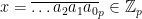${x = \overline{\dots a_2 a_1 a_0}_p \in \mathbb Z_p}$ then

$\displaystyle \sum_{k=0}^\infty a_k p^k \quad\text{converges to } x.$

Indeed, the ${n}$ th partial sum is divisible by ${p^n}$ , hence the partial sums approach ${x}$ as ${n \rightarrow \infty}$ .

While the definitions are all the same, there are some changes in properties that should be true. For example, in ${\mathbb Q_p}$ convergence of partial sums is simpler:

Proposition 15 ( ${|x_k|_p \rightarrow 0}$ iff convergence of series)

A series ${\sum_{k=1}^\infty x_k}$ in ${\mathbb Q_p}$ converges to some limit if and only if ${\lim_{k \rightarrow \infty} |x_k|_p = 0}$ .

Contrast this with ${\sum \frac1n = \infty}$ in ${\mathbb R}$ . You can think of this as a consequence of strong triangle inequality. Proof: By multiplying by a large enough power of ${p}$ , we may assume ${x_k \in \mathbb Z_p}$ . (This isn’t actually necessary, but makes the notation nicer.)

Observe that ${x_k \pmod p}$ must eventually stabilize, since for large enough ${n}$ we have ${\left\lvert x_n \right\rvert_p < 1 \iff \nu_p(x_n) \ge 1}$ . So let ${a_1}$ be the eventual residue modulo ${p}$ of ${\sum_{k=0}^N x_k \pmod p}$ for large ${N}$ . In the same way let ${a_2}$ be the eventual residue modulo ${p^2}$ , and so on. Then one can check we approach the limit ${a = (a_1, a_2, \dots)}$ . $\Box$

Here’s a couple exercises to get you used to thinking of ${\mathbb Z_p}$ and ${\mathbb Q_p}$ as metric spaces.

Exercise 16 ( ${\mathbb Z_p}$ is compact)

Show that ${\mathbb Q_p}$ is not compact, but ${\mathbb Z_p}$ is. (For the latter, I recommend using sequential continuity.)

Exercise 17 (Totally disconnected)

Show that both ${\mathbb Z_p}$ and ${\mathbb Q_p}$ are totally disconnected: there are no connected sets other than the empty set and singleton sets.

3.3. More fun with geometric series

While we’re at it, let’s finally state the ${p}$ -adic analog of the geometric series formula.

Proposition 18 (Geometric series)

Let ${x \in \mathbb Z_p}$ with ${\left\lvert x \right\rvert_p < 1}$ . Then

$\displaystyle \frac{1}{1-x} = 1 + x + x^2 + x^3 + \dots.$

Proof: Note that the partial sums satisfy ${1 + x + x^2 + \dots + x^n = \frac{1-x^n}{1-x}}$ , and ${x^n \rightarrow 0}$ as ${n \rightarrow \infty}$ since ${\left\lvert x \right\rvert_p < 1}$ . $\Box$

So, ${1 + 3 + 3^2 + \dots = -\frac{1}{2}}$ is really a correct convergence in ${\mathbb Z_3}$ . And so on.

If you buy the analogy that ${\mathbb Z_p}$ is generating functions with base ${p}$ , then all the olympiad generating functions you might be used to have ${p}$ -adic analogs. For example, you can prove more generally that:

Theorem 19 (Generalized binomial theorem)

If ${x \in \mathbb Z_p}$ and ${\left\lvert x \right\rvert_p < 1}$ , then for any ${r \in \mathbb Q}$ we have the series convergence

$\displaystyle \sum_{n \ge 0} \binom rn x^n = (1+x)^r.$

(I haven’t defined ${(1+x)^r}$ , but it has the properties you expect.) The proof is as in the real case; even the theorem statement is the same except for the change for the extra subscript of ${p}$ . I won’t elaborate too much on this now, since ${p}$ -adic exponentiation will be described in much more detail in the next post.

3.4. Completeness

Note that the definition of ${\left\lvert \bullet \right\rvert_p}$ could have been given for ${\mathbb Q}$ as well; we didn’t need ${\mathbb Q_p}$ to introduce it (after all, we have ${\nu_p}$ in olympiads already). The big important theorem I must state now is:

Theorem 20 ( ${\mathbb Q_p}$ is complete)

The space ${\mathbb Q_p}$ is the completion of ${\mathbb Q}$ with respect to ${\left\lvert \bullet \right\rvert_p}$ .

This is the definition of ${\mathbb Q_p}$ you’ll see more frequently; one then defines ${\mathbb Z_p}$ in terms of ${\mathbb Q_p}$ (rather than vice-versa) according to

$\displaystyle \mathbb Z_p = \left\{ x \in \mathbb Q_p : \left\lvert x \right\rvert_p \le 1 \right\}.$

(Remark for experts: ${\mathbb Q_p}$ is a field with ${\nu_p}$ a non-Arcihmedian valuation; then ${\mathbb Z_p}$ is its valuation ring.)

Let me justify why this definition is philosophically nice.

Suppose you are a numerical analyst and you want to estimate the value of the sum

$\displaystyle S = \frac{1}{1^2} + \frac{1}{2^2} + \dots + \frac{1}{10000^2}$

to within ${0.001}$ . The sum ${S}$ consists entirely of rational numbers, so the problem statement would be fair game for ancient Greece. But it turns out that in order to get a good estimate, it really helps if you know about the real numbers: because then you can construct the infinite series ${\sum_{n \ge 1} n^{-2} = \frac16 \pi^2}$ , and deduce that ${S \approx \frac{\pi^2}{6}}$ , up to some small error term from the terms past ${\frac{1}{10001^2}}$ , which can be bounded.

Of course, in order to have access to enough theory to prove that ${S = \pi^2/6}$ , you need to have the real numbers; it’s impossible to do serious analysis in the non-complete space ${\mathbb Q}$ , where e.g. the sequence ${1}$ , ${1.4}$ , ${1.41}$ , ${1.414}$ , \dots is considered “not convergent” because ${\sqrt2 \notin \mathbb Q}$ . Instead, all analysis is done in the completion of ${\mathbb Q}$ , namely ${\mathbb R}$ .

Now suppose you are an olympiad contestant and want to estimate the sum

$\displaystyle f_p(x) = \sum_{k=1}^{p-1} \frac{1}{(px+k)^2}$

to within mod ${p^3}$ (i.e. to within ${p^{-3}}$ in ${\left\lvert \bullet \right\rvert_p}$ ). Even though ${f_p(x)}$ is a rational number, it still helps to be able to do analysis with infinite sums, and then bound the error term (i.e. take mod ${p^3}$ ). But the space ${\mathbb Q}$ is not complete with respect to ${\left\lvert \bullet \right\rvert_p}$ either, and thus it makes sense to work in the completion of ${\mathbb Q}$ with respect to ${\left\lvert \bullet \right\rvert_p}$ . This is exactly ${\mathbb Q_p}$ .

4. Solving USA TST 2002/2

Let’s finally solve Example~1, which asks to compute

$\displaystyle f_p(x) = \sum_{k=1}^{p-1} \frac{1}{(px+k)^2} \pmod{p^3}.$

Armed with the generalized binomial theorem, this becomes straightforward.

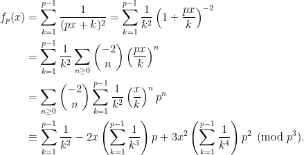
$\displaystyle \begin{aligned} f_p(x) &= \sum_{k=1}^{p-1} \frac{1}{(px+k)^2} = \sum_{k=1}^{p-1} \frac{1}{k^2} \left( 1 + \frac{px}{k} \right)^{-2} \\ &= \sum_{k=1}^{p-1} \frac{1}{k^2} \sum_{n \ge 0} \binom{-2}{n} \left( \frac{px}{k} \right)^{n} \\ &= \sum_{n \ge 0} \binom{-2}{n} \sum_{k=1}^{p-1} \frac{1}{k^2} \left( \frac{x}{k} \right)^{n} p^n \\ &\equiv \sum_{k=1}^{p-1} \frac{1}{k^2} - 2x \left( \sum_{k=1}^{p-1} \frac{1}{k^3} \right) p + 3x^2 \left( \sum_{k=1}^{p-1} \frac{1}{k^4} \right) p^2 \pmod{p^3}. \end{aligned}$

Using the elementary facts that ${p^2 \mid \sum_k k^{-3}}$ and ${p \mid \sum k^{-4}}$ , this solves the problem.

2 thoughts on “A trailer for p-adic analysis, first half: USA TST 2003”

kayak October 20, 20182:03 AM Reply

Isn’t Chaper 6B of SfTB about Probabilistic method … I suppose you mean 3A ?

Also this looks way more understandable/approachable than addendum 3A (which I don’t understand even a para) — thanks a lot for writing this !

When the second half is going to be released :D ?

LikeLike
1. Evan Chen (陳誼廷) October 20, 201810:17 AM Reply
  
  Yep, 3A. Thanks. The second half should be out in a few weeks.
  
  LikeLike

A trailer for p-adic analysis, first half: USA TST 2003

1. Motivation

2. Algebraic perspective

2.1. Definition of ${\mathbb Z_p}$

2.2. Base ${p}$ expansion

2.3. Constructing ${\mathbb Q_p}$

3. Analytic perspective

3.1. Definition

3.2. Ultrametric space

3.3. More fun with geometric series

3.4. Completeness

4. Solving USA TST 2002/2

Published by Evan Chen (陳誼廷)

2 thoughts on “A trailer for p-adic analysis, first half: USA TST 2003”

Leave a Reply Cancel reply

1. Motivation

2. Algebraic perspective

2.1. Definition of

2.2. Base expansion

2.3. Constructing

3. Analytic perspective

3.1. Definition

3.2. Ultrametric space

3.3. More fun with geometric series

3.4. Completeness

4. Solving USA TST 2002/2

Share:

Like this:

Related

Published by Evan Chen (陳誼廷)

2 thoughts on “A trailer for p-adic analysis, first half: USA TST 2003”

Leave a Reply Cancel reply

2.1. Definition of ${\mathbb Z_p}$

2.2. Base ${p}$ expansion

2.3. Constructing ${\mathbb Q_p}$